CodeLinker - Model 1.0 -RNA-Seq Differential Expression Data Analysis Software

CodeLinker is a user-friendly and powerful desktop software program for analyzing your microarray data with powerful analyses and rich vizualizations.  It`s a unique paradigm where every analysis is an experiment that makes your work really flow. And for those experiments where you are looking for concordance between your RNA-Seq and Microarray data, shouldn`t you have concordance in your analysis software as well?  You can with CodeLinker.

With CodeLinker, your functional genomics experimentation doesn’t stop at the bench. Using this paradigm, you can take your data and look at it using different algorithms and visualizations. Whether you are working with microarrays or RNA-Seq differential expression results from Cuffdiff, CodeLinker can give you the insight you are looking for from your datasets. Store all your analyses and visualizations in CodeLinker, you don`t even need to remember to save the project, it’s done automatically.

NORMALIZATION

Technical error can creep into the best planned and executed experiments. As a pre-requisite to analysing your data, you may need to put your data on a single scale of variation. So to help you level the playing field, CodeLinker has a collection of techniques for correcting non-biological variation between samples.

CLUSTERING

The goal of expression analysis with CodeLinker is to explore your expression profiles in order to make biological inferences about your dataset. It doesn`t matter whether your point of view is from that of the genes or the samples you are working with. CodeLinker’s collection of tools assists you in doing that. Clustering is the name given to the task of grouping items together in such a way that those within the cluster are more similar to each other than those in other clusters. Choose from the classical clustering algorithm or algorithms rooted in agglomerative methods or methods based on the similarity between neighbors. With Codelinker, you have wide choices. While the methods may vary, the end goal is to uncover patterns of expression that give you insight into the problem you are studying, perhaps even uncovering patterns you did not know existed.  

DISTANCE METRICS

Comparison of expression profiles requires the ability to measure how similar the genes or samples in question are. In order to accomplish this, ten distance measures are available in CodeLinker covering a wide variety of scenarios. Seven distance metrics are devoted to the measurement between the data points in a cluster and three separate distance measurements are devoted to the distance between the clusters.

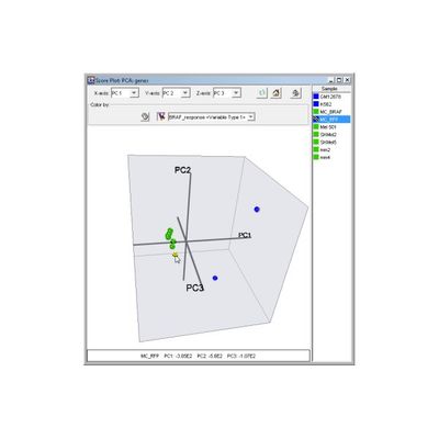
PRINCIPAL COMPONENT ANALYSIS

Typically, gene expression datasets are large and complex with large numbers of interrelationships. This is true whether you have generated your data using RNA-Seq for differential expression analysis or you have used microarrays. With large numbers of genes and the potential for many samples, one of the best ways to proceed is to reduce the dimension space you are exploring using Principal Component Analysis (PCA). With no parameters to set, this is one of the easiest ways to begin your analysis and reduce complexity, while still computing a new, much smaller set of uncorrelated variables which best represent the original data.

VISUALIZATIONS

CodeLinker implements visualization at every step starting from the moment you import your data. CodeLinker offers you plots which let you visually determine those genes that show significant induction or repression through to looking at expression profiles when you are exploring the entirety of your samples or genes. Whether you want to visualize the exemplar profile for the clusters generated, or display the profiles of individual members within a cluster, CodeLinker has plots which really highlight clustering relationships.

DATA PREDICTION

What makes CodeLinker unique is its set of data prediction tools, especially SLAM which is something you won’t find anywhere else – it’s an association mining tool. This means that it can search through your expression data, exploring the expression profiles with the goal of creating a list of interesting genes. Quite simply put, the algorithm will find sets of gene expression values which co-occur more frequently within each dataset. Together with tools to help you identify patterns of gene expression that characterize different responses to stimuli, disease states, or drug treatments, you can then put this knowledge to work testing hypotheses.

CLUSTERING

Clustering is a type of multivariate statistical analysis that is widely used in biology to place biological samples or genes into separate groupings based on their statistical behavior. The main objective is to find similarities between experiments or genes. CodeLinker provides you with a set of tools with which to cluster and explore your data to assist in understanding the relationships that might exist in them.

The clustering techniques include K-Means clustering which generates a specific number of flat (non-hierarchical) clusters. Jarvis-Patrick clustering is a clustering method based on similarity between neighbors determined by using a distance metric. One or more Neighbors in Common are used to judge the cluster membership of the objects under study. Agglomerative hierarchical clustering is a bottom-up clustering method where clusters have sub-clusters, which in turn have sub-clusters, etc. The classic example of this is species taxonomy. The  Self-Organizing Map (SOM)  is a clustering algorithm that is used to map a multi-dimensional dataset onto a (typically) two-dimensional surface. This surface (a map) is an ordered interpretation of the probability distribution of the available genes/samples of the input dataset.

The distance metrics specify how the distance between data points in the clustering input is measured. CodeLinker gives you a wide choice of metrics to choose from. You can choose from the standard Euclidean (as-the-crow-flies) distance or the Manhattan (city block) distance. Where you want to cluster genes or samples with similar behavior, use the Pearson Correlation Coefficient.  If you want to cluster genes that are highly correlated and those that are anti-correlated, use the Squared Pearson Correlation Coefficient. With data that does not show dramatic expression differences in any samples, you may use the Chebychev distance. Use the Euclidean Squared distance in cases where you would use regular Euclidean distance in Jarvis-Patrick or K-Means clustering and, finally, you may use the Spearman Correlation to cluster together genes whose expression profiles have similar shapes or show similar general trends (e.g. increasing expression with time), but whose expression levels may be very different.

To visualize your analyses, there are specialized plots tuned for the algorithms you used to perform the original analysis. Each plot type can be customised and you can export your plot in PNG, SVG, or PDF formats.

PRINCIPAL COMPONENT ANALYSIS

Principal Component Analysis (PCA) is an unsupervised or class-free approach to finding the most informative or explanatory features in a dataset. In particular, PCA substantially reduces the complexity of data in which a large number of variables (e.g. thousands) are interrelated, such as in large-scale gene expression data obtained across a variety of different samples or conditions. CodeLinker provides two options for PCA analysis:  Orientation by Genes or Orientation by Samples, the former of which allows you to distinguish sample sets while the latter allows you to distinguish gene sets.

To visualize your analyses, there are specialized plots tuned for the algorithms you used to perform the original analysis. Each plot type can be customised and you can export your plot in PNG, SVG, or PDF formats.

SLAM, IBIS and ANN – Prediction Tools

RNA-Seq has brought about a revolution in the study of gene expression. It is now possible to study the expression landscape of virtually any organism even if a species specific microarray is not readily available. However, each technological innovation brings about new problems, and for RNA-Seq, it is with the sheer quantity of data that is produced. Eyeballing it is no longer an option, and Excel will not cope. While there are powerful tools out there, they are often command-line driven, and tight deadlines mean you don`t have the time to learn how to use yet another package on the command line. With Sequencher, we gave you the ability to run your NGS alignments and gene expression differential analysis through an intuitive GUI. Now with CodeLinker, we are giving you the same ability, an easy-to-use GUI with which to analyse your RNA-Seq data in depth, from your desktop.

Imagine that you are studying a disease but the expression data you have so far, while indicative, are not diagnostic. Starting with RNA-Seq differential expression results, you can use CodeLinker to find new patterns of gene expression using SLAM and ANN that are predictive of the disease you are studying. The data you have contains hidden associations (sets of genes and expression values), and with the help of SLAM/ANN, or IBIS, you can uncover these associations.

Sub-Linear Association Mining (SLAM) searches your gene expression data looking for sets of features, that is to say patterns of expression, which occur together more than might be expected by chance and discriminate between the values of any variable (gene). Once you have exposed these associations, you can then use them to train the ANN or Artificial Neural Network and then go on to classify test data. While they say that nothing good comes from a committee, that is definitely not the case when you use committees of networks. This method will generate more accurate results than would be obtained from just a single neural network. Having taught the ANN with the training data you provided, you are now ready to analyse your test data. The results can be displayed in the graphically rich Classification Plot, giving each sample in your test set a classification – predicted, true class (something different from your original classification), or unknown. This will assist in confirming or refuting your hypothesis concerning the data.

Suppose you are studying the response of certain cell types to a drug treatment. Just as you told Cuffdiff the conditions for each sample (drug dose, tissue type, phenotype), you can use the same classifications with CodeLinker. Two sets of information are imported into CodeLinker – a set of expression data, and the list of tissues and their responses to the drug treatment. These can be explored using the Integrated Bayesian Inference System (IBIS).

The IBIS classifier is a method that uses Bayesian probabilities to look at the patterns in your data. IBIS offers powerful search capabilities into your data. It can identify non-linear and combinatorial patterns of gene expression that characterize different toxicity responses, disease states, or treatment outcomes. Furthermore, it can be used to build classifiers that can identify these patterns in new samples. It can also be used as a search tool to identify single genes and small gene sets that show interesting expression patterns relative to the sample classification.

These are imported into CodeLinker, then a Linear Discriminant Analysis search is performed which evaluates the accuracy of each gene when used as linear discriminator i.e. it has the ability to separate the data into two or more classes. Genes with lower Mean Square Errors (MSEs) reflect how well the data matches the linear model. Choosing one of these, you can then display the results of the analysis on a plot whose background color gradient represents the classification that IBIS discovered; the plot displays the gene expression and spots with colors representing the initial classification that you gave. You can see with ease whether the genes you have focussed on fit the pattern you expected or are exposing new and unexpected correlations. With the 2D plot, you can explore the putative relationships between pairs of genes and find new relationships that divide along the line of your initial classification. Spotting the false positives and false negatives is as simple as looking at the colors of the spots in relation to the colored background on the graph. For more complex data where there is no linear relationship, CodeLinker provides you with the ability to perform 2D Linear Discriminant Analysis or even Quadratic or Gaussian Discriminant Analysis.