Why your Groundwater Model is Already Out of Date (And what to do About it)

That`s not a criticism of the consultants who built them. It`s a structural problem. The science of groundwater contamination modeling has advanced considerably over the past two decades - ensemble calibration methods, automated parameter estimation, uncertainty quantification. None of it has meaningfully reached standard practice.

A 2024 study of operational groundwater modeling workflows found the gap plainly: "Important academic advances in groundwater modelling over the past two decades have not translated into practical application. Uncertainty quantification is rarely undertaken."(4) None of the workflows analyzed included any form of automated data assimilation.(4)

This article explains why that gap exists, what it costs, and how automated groundwater modeling is beginning to close it.

‍What Groundwater Contamination Modeling Actually Does

When regulators ask where a contamination plume is now, where it will be in ten years, and when concentrations will cross thresholds near neighboring receptors - those questions cannot be answered by measurement alone. Tools like GWSDAT provide excellent spatiotemporal analysis of where a plume has been. Predicting future behavior requires a numerical model.

A groundwater numerical model subdivides the subsurface into a three-dimensional grid of cells - typically 50,000 to 500,000 for a contaminated site - each representing a discrete volume of earth.(5) Every cell is assigned hydraulic conductivity, porosity, contaminant transport properties, and biodegradation rates. The model solves physics equations across the entire grid, producing simulated groundwater levels and contaminant concentrations at every point in the domain.

The challenge is calibration. Hydraulic conductivity alone can vary by three to five orders of magnitude within a single site.(6) Fine-grained clay lenses sitting next to coarse gravel channels, buried infrastructure nobody mapped, fill material with unknown properties - all create flow pathways the model needs to capture while the sparse well network can barely detect them.

A typical contaminated site model contains 50,000 to 500,000 grid cells but is calibrated against data from only 10 to 30 monitoring wells.(5) That ratio - vastly more unknowns than observations - is not a solvable problem in the traditional sense. It is a fundamentally underdetermined problem.

Why a Single "Best Fit" Model Is the Wrong Answer

The standard response to this underdetermined problem is to calibrate once and report a single result. A consultant adjusts model parameters until simulated water levels match measured values, runs one simulation, and delivers one prediction.

That prediction looks precise. It isn`t.

With sparse data - twenty wells spread across a multi-hectare site - many different parameter combinations can produce equally good fits to the observations. A high-conductivity zone in one location could be offset by a low-conductivity zone elsewhere; both configurations match the measured water levels. This is what hydrogeologists call the Curse of Equifinality: a single "best fit" model conceals many other equally plausible representations of the subsurface.

"The plume will reach the property boundary in 12 years" sounds actionable. But it hides the question that actually drives capital planning and regulatory negotiation: what is the confidence level of that assessment?

Ensemble methods address this by treating calibration as a probabilistic exercise rather than a point estimation problem. Instead of calibrating once, calibration is performed multiple times across hundreds of different parameter sets. Each produces a slightly different model. The spread across all predictions generates uncertainty bounds at every grid cell - a measured range reflecting how much the data actually constrains the answer.

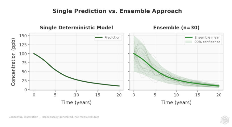
The resulting output - "there is a 90% probability the plume reaches the property boundary between 8 and 16 years" - is less tidy than a single number. It is far more useful for decisions that involve real money and real regulatory consequences.

Where Most Industry Practice Sits Today

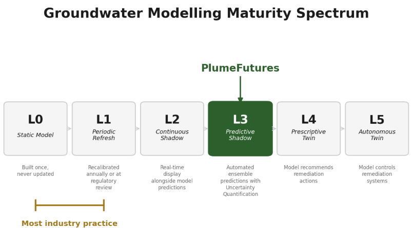
Most contaminated site work operates at what might be called Level 0 or Level 1 on a groundwater modeling maturity spectrum:

Level 0 - Static model. Built once by a consultant, delivered as a PDF, never updated. The model reflects conditions at the time of construction. When conditions change - new sampling data arrives, remediation progresses, seasonal patterns shift - the model doesn`t.

Level 1 - Periodic refresh. Model recalibrated annually or at regulatory five-year reviews. Still manual. Still delivers periodic static snapshots rather than continuously updated predictions.

Level 2 - Continuous shadow. Real-time sensor data displayed alongside model predictions. Humans compare the two and decide when recalibration is warranted.

Level 3 - Predictive shadow. Automated recalibration incorporating new data as it arrives. Ensemble-based predictions with uncertainty quantification and forward projections under multiple remediation scenarios simultaneously.

The tools required to reach Level 3 already exist and are free. MODFLOW6, the USGS groundwater simulation standard accepted by regulators across North America, has been open source since the 1980s.(7) PEST++, the parameter estimation software that enables ensemble-based calibration, is also free and open source. The barrier is not technology. It is operational: nobody has automated the pipeline that turns raw site data into a calibrated, uncertainty-quantified groundwater model and keeps it current as new data arrives.

The Data Problem: What Quarterly Sampling Actually Produces

Standard practice across the roughly 60,000 sites in the EPA`s LUST backlog is quarterly grab sampling - producing two to four concentration measurements per monitoring well per year.(1) At a 40-well site, that equals 80 to 160 total data points annually. Large contaminated sites can spend $200,000 per year on this sampling;(8) smaller sites typically spend $10,000 to $50,000.(9)

That data poverty has a direct statistical consequence for plume management.

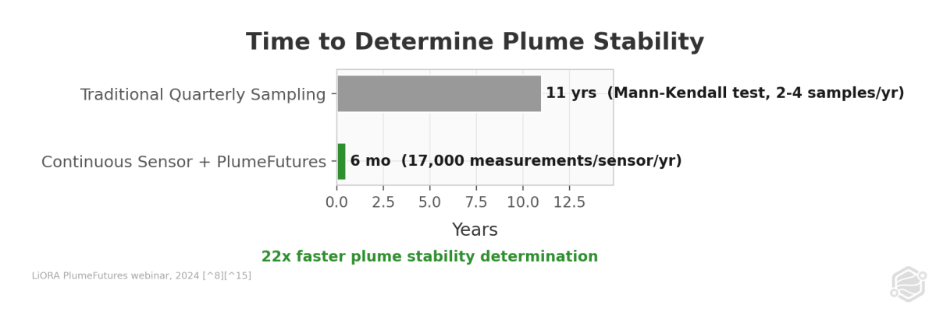
The Mann-Kendall trend test - the standard non-parametric method regulators use to determine whether a contaminant plume is stable, growing, or shrinking - requires substantial data to reach meaningful conclusions. With two to four samples per well per year, the test cannot reliably distinguish real trends from sampling noise for 10 to 12 years.(8) It is not a flaw in the test. It is a statistical power problem. You simply don`t have enough observations.

The consequence is that plume stability determinations - the metric that tells regulators a site is heading toward closure - take a decade by design under standard monitoring practice.

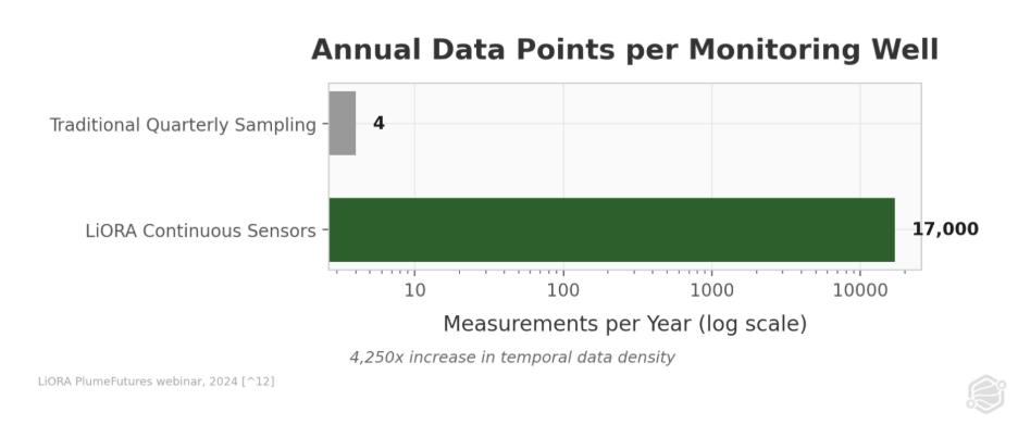
Continuous sensor data changes this math entirely. LiORA`s NDIR (Non-Dispersive Infrared) subsurface gas sensors produce approximately 17,000 measurements per sensor per year, sampling every 30 minutes.(8) Across a 40-sensor network, that equals 680,000 data points annually versus 160 from quarterly sampling at the same site. With that data density feeding an automated groundwater model, plume stability can be determined within approximately six months rather than ten to twelve years.(8)

The model isn`t smarter. The data is denser.

What Automated Groundwater Modeling Produces

PlumeFutures, LiORA`s automated groundwater modeling platform, is built on MODFLOW6 - the same simulator regulators already trust - with an automated pipeline that handles grid construction, parameter estimation, ensemble calibration, and forward projection.

What goes in: Historical sampling records, Phase II Environmental Site Assessment reports, and digital elevation models. No sensors are required to initialize a model. When LiORA`s continuous sensors are deployed, the platform additionally ingests 17,000 measurements per sensor per year to continuously refine calibration.(8)

What comes out: Twenty-year forward projections of contaminant plume migration, evaluated simultaneously under three remediation scenarios:

• Baseline - no intervention. The "do nothing" trajectory used as a reference for comparison.

• NSZD (Natural Source Zone Depletion) - enhanced natural biodegradation. When LiORA sensors are deployed, NSZD rates are calculated from measured soil gas concentration gradients rather than literature estimates, making the scenario site-specific rather than generic.

• Biostimulation - active remediation via nutrient or electron acceptor injection to stimulate microbial degradation of petroleum hydrocarbons.

Every prediction includes uncertainty bounds - not a single line on a graph, but a distribution of outcomes reflecting parameter uncertainty across the ensemble of calibrated models.

Three core decision metrics drive the outputs:

1. Time-to-stability. When will the plume stop changing? A plume is considered stable when concentration and area change by less than 1% per year.(10) This determines whether a site is heading toward closure or still evolving.

1. Time-to-fence-line. When will contamination reach the property boundary or nearest sensitive receptor? This is the metric that triggers regulatory intervention and drives capital allocation decisions.

1. Portfolio triage. In a typical portfolio of contaminated sites, approximately 90% are stable or naturally attenuating and need monitoring but not intervention. The remaining 10% have migrating or growing plumes that require action.(8) Identifying that 10% without commissioning individual studies for every property is the portfolio-scale problem automated modeling was built for.

What This Means for Site Managers

When sensors are deployed, PlumeFutures performs monthly data fusion. Each month, new sensor data is incorporated into the existing calibrated model. The model recalibrates against both historical and new observations. Forward projections regenerate with updated parameters.

Over time, uncertainty generally decreases in areas with good sensor coverage. Where it increases - where new data conflicts with prior assumptions - that is the model surfacing what the original site characterization missed. Buried infrastructure deflecting flow. Geological heterogeneity not captured in initial boring logs. That increase in uncertainty may be the most valuable output in some cases: it tells you where to look next.

For site managers and environmental engineers, the practical shift is from "model it once and hope" to "model it continuously and know." Plume stability determination moves from a decade-long waiting game to a six-month assessment, which means closure conversations with regulators can start years earlier. For anyone managing a portfolio of 20 or 50 or 200 contaminated sites, the question "which ones actually need attention this quarter?" becomes answerable without a separate study for each property.

What Automated Groundwater Modeling Cannot Do (Yet)

Environmental professionals detect overselling immediately. Automated groundwater modeling has clear limits that are worth stating directly.

It is not a digital twin. Automated modeling at Level 3 - ensemble predictions with uncertainty quantification - does not close the loop. It does not recommend remediation actions and does not execute them. The predictions inform human decisions. Moving to Level 4, prescriptive models that recommend specific interventions, requires regulatory frameworks for model-driven decision-making that do not yet exist in most jurisdictions.

It does not eliminate subsurface uncertainty. More data reduces epistemic uncertainty - things you could know but don`t yet. Some uncertainty is irreducible. The subsurface will always have more heterogeneity than any practical number of sensors can measure. The ensemble approach quantifies this honestly rather than hiding it behind a single prediction that implies more precision than the data supports.

Spatial resolution is bounded by well locations. Continuous sensors provide extraordinary temporal density - 17,000 measurements per year per location - but spatial density does not change. The space between wells is interpolated. More wells improve spatial resolution. Sensors solve the temporal problem, not the spatial one.

Not every site type is equally well-served. The automated pipeline is built for petroleum hydrocarbon contamination at sites with sufficient historical data to initialize a model. Complex mixed-contaminant sites, fractured bedrock geology, or sites with minimal data histories require more manual expert interpretation than the automated pipeline currently handles.

Regulatory acceptance is evolving. MODFLOW-based models are widely accepted because MODFLOW is the USGS standard. Continuously updated, automated models are newer territory. In most jurisdictions today, this is a supplemental use situation - the monitoring requirement is not going away, but the monitoring data becomes more useful and the resulting predictions more defensible.